Animating HMI values and system performance
In this post we dive in to visualizing some data on the HMI that comes over a communication interface. At the same time we will take a look at “system performance” and the perception of “system performance”.
Take a look at this video first, can you tell which system is performing better? System 1 or System 2?
If you said System 2 you would be wrong. Both visualizations are running on the same PLC and using the same data. Let us see what is happening here!
System performance is in the eye of the beholder
Most of the time a system is perceived to be slow if the user does not get any continuous feedback. Even worse, performance evaluation will be bad if the values change infrequently on the screen e.g. stuttering.
I heard a story about a computer in the 80s. Most of the computers of that time had long boot processes as they were checking memory and other OS critical things. These boot processes took something like minutes to complete before you were able to use the computer. This computer in question was no different but it had one advantage. It had a splash screen with running bars with the text “Loading”. Believe it or not, the computer was selling better than the others and was perceived to be faster than the rest, even though it took the same amount of time to boot as the others. Other computers looked like they have hanged, giving no feedback to the user they were doing anything in the background.
Similar thing happens to the data presented on the HMI screens.
Technical problem
To make something look nice and smooth to the human eye, we need a frame rate of about 24 frames per second. If we plug in a variable coming from the field directly to the visualization element, in order to make it look smooth, we would need to increase the data rate quite significantly.
Lets take ModbusTCP for example, running at 500ms cycle and the data a simple sine curve connected to the analog input card. We can assume the sine is sampled by the card extremely well and what we get into the PLC is a perfect curve. This data is transmitted to the HMI by ModbusTCP at the specified rate. In this case, our sampling rate of the signal is no longer perfect as we are “sampling” it every 500ms when sending it. The receiving end still has to receive the data and process it but for the purpose of this post we will assume the HMI receives new data every 100ms. The sine curve now becomes “blocky” and will be shown to the user as such.
The data would look something like this:
At 500ms modbus update rate we get 2 FPS on the screen. This is far from perfect. In order to get it up to 24 FPS, the modbus update rate would need to be 24ms. The poor PLC would be sending the data and that is the only thing it could do. Slower data rates further exacerbate the problem however.
Animation to the rescue
It is not necessary to increase the data rate to 24 ms, we just animate it. In this way we can get even higher frame rates than 24 FPS. We just need to run the HMI visualization faster than the incoming data and approximate the “missing data”. This wizardry of animation is included in many HMI vendors that make life easier, but there are also an equal amount of them that don’t. Here are some ideas on how to do animation by your self with the usual pros and cons.
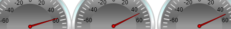
I use Codesys for most of my posts and this one is no different. Here is a nice video of the arrow scales approximating the data coming from an imaginary Modbus line, running at 500ms update rate.
Animation however comes with a negative side effect as our animated data is decoupled slightly from the source. Solutions I present in this post introduce either a delayed response value or shifting in phase of the signal. This means that, even if it looks faster, we are just fooling our eyes. All solutions will also spend CPU time so this should be used only where necessary.
Animating using inertia (a simple ramp)
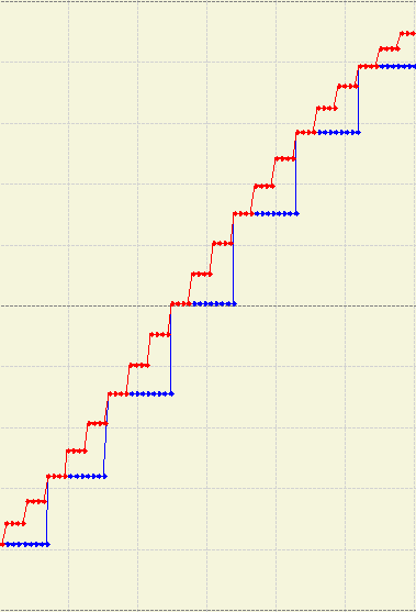
Any value can have inertia. The communicated data from the modbus has no inertia, meaning the data in the destination changes instantly upon receiving new data. This is the main reason of jitter. To overcome this, we can introduce a simple ramp function with a fixed slope to introduce inertia. Inertia is defined as resistance to change so by ramping the communicated value we can make the needle move smoothly across the screen.
If the communicated data is predictable and its rate of change is fixed, the output signal of the ramp might look something like this.
However, the communicated data depends on the real world values which are unpredictable. The simple ramp approach fails miserably when the communicated data changes rapidly. Then the output signal of the ramp might be very late or not even reaching the peaks, giving wrong information.
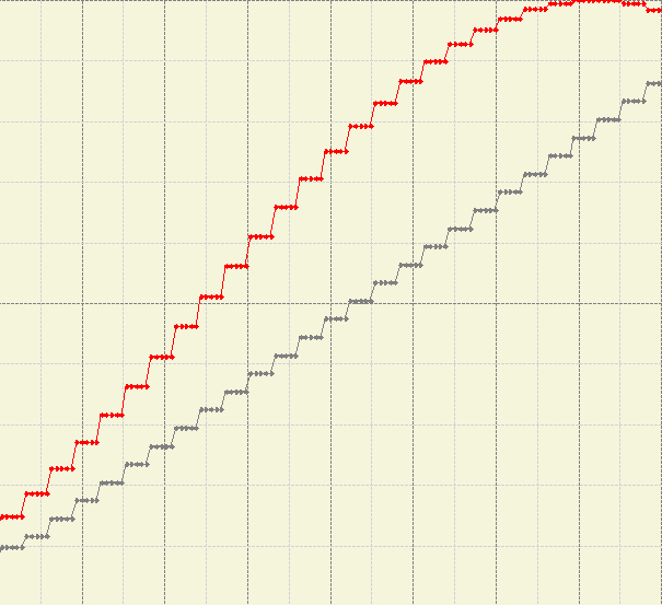
We will tackle this problem in the next chapter.
Here is an implementation of a simple ramp and its use in this context.
FUNCTION simpleRamp : REAL
VAR_INPUT
    oldValue : REAL;
    spValue : REAL;
    slope : REAL;
END_VAR

BEGIN IMPLEMENTATION
    (*Increment or decrement*)
    (*After incrementing or decrementing, check if we went outside spValue*)
    IF spValue > oldValue THEN
        simpleRamp := MIN(oldValue + slope, spValue);
        RETURN;
    ELSIF spValue < oldValue THEN
        simpleRamp := MAX(oldValue - slope, spValue);
        RETURN;
    END_IF
    (*Value is the same*)
    simpleRamp := spValue;
    RETURN;
END_IMPLEMENTATION
(*Using a ramp function (inertia)*)
inertialData := simpleRamp(inertialData, txData, inertialSlope);
Animating using dynamic inertia (still a simple ramp)
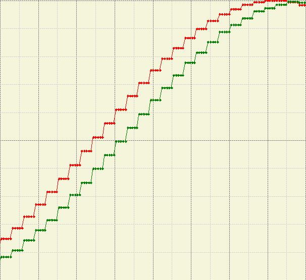
There is a simple solution to the rate of change of the communicated data. We simply calculate the difference between two points in time. Once we receive new data we apply the ramp and store the value in memory. However, if we would leave it like this, the ramp would again produce the same output value as the communicated data, producing no animation effect. We have to multiply the difference of the signal with a scaler. The scaler, just a number between 0 and 1, is responsible for creating the interpolated points in between. At 1, there will be no interpolation points, at 0.5 there will be two, at 0.3333 there will be three and so on. Because the communicated data rate of change is dynamic so are our interpolation points and the distances between. In translation, if the rate of change is high, so will be the slope of the ramp between points. If the rate of change is low so will be the slop of the ramp. The output value of the ramp will closely follow the curves of the real world signal with a slight offset in phase.
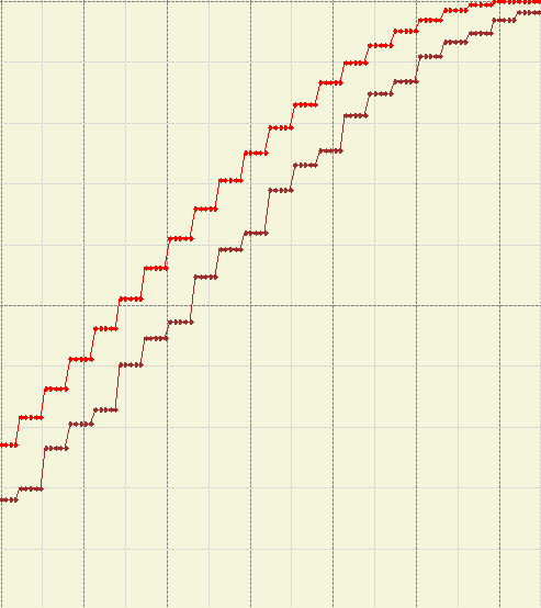
Here is how that might look like.
Here is an example of calculating the difference of the incoming signals rate of change.
(*Differential ramp speed (dynamic inertia)*)
 (*Calculate the difference between new and old data*)
IF txDataOld <> txData THEN
   dtRaw := txData - dynInertialData;
   txDataOld := txData;
END_IF
dynInertialData := simpleRamp(dynInertialData, txData, ABS(dtRaw)* dynInertiaScaler);
Using the simple ramp approach might not be that good if memory and CPU time is crucial. This is especially the case if there are a lot of values that need this kind of animation. Let us see in the next chapter how we could optimize this.
Animating using linear interpolation (Lerp)
According to Wikipedia:
In mathematics, linear interpolation is a method of curve fitting
using linear polynomials to construct new data points within the
range of a discrete set of known data points.
This is exactly what our approach using dynamic inertia is doing. Taking two points in time and applying them with a curve, or a set of curves, depending how many data points we want to use.
Pseudo code from Wikipedia:
// Precise method, which guarantees v = v1 when t = 1.
// This method is monotonic only when v0 * v1 < 0.
// Lerping between same values might not produce the same value
float lerp(float v0, float v1, float t) {
  return (1 - t) * v0 + t * v1;
}
This can be written in structured text the same way, as a function that returns a real.
FUNCTION Lerp : REAL
VAR_INPUT
    v0: REAL;
    v1 : REAL;
    t : REAL;
END_VAR
BEGIN IMPLEMENTATION
    Lerp := (1-t) * v0 + t * v1;
END_IMPLEMENTATION

//And the call
(*Linear interpolation*)
lerpData := Lerp(lerpData, txData, lerpScaler);
This approach uses much less of the CPUs time and memory so it should be better for uses where there is a lot of Lerping necessary.
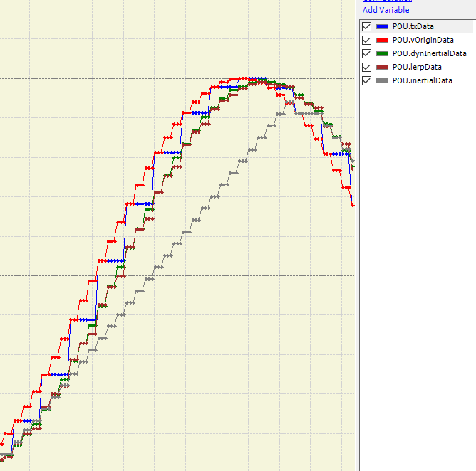
When applied, the output signal would look something like this:
From the trace we can see that the lerp curve doesnt perfectly match the real world value but it is good enough for most cases. Especially when it is more efficient than the other solutions I have found. It also solves the variable data rate problem at the same time and it keeps the amount of parameters quite low.
This implementation can also be called Exponential Moving Average Low Pass filter.
Side to side comparisons